DIMES US2 Cruise Summary - Final Report15 January to 5 March 2010
5 March 2010
R/V Thomas G. Thompson
Cruise TN246
Cruise TN246 is coming to a successful conclusion, with all science stations completed and the ship heading into Punta Arenas through the eastern branch of the Strait of Magellan. The following summary works backwards through the cruise, for novelty.
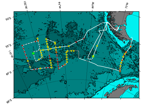
Fig. 1. Ship Track and Stations. CTD/LADCP (black dots), HRP (yellow dots), DMP deployment (red triangles) occupied during TN246. The green stars mark the positions of the two moorings that were also deployed during the cruise. Samples were taken for tracer at all but the Drake Passage stations.
The last phase of the cruise supported a series of 13 fine- and microstructure stations from south to north across Drake Passage, using the HRP, the DMP, and 3 expendable microstructure profilers (Fig. 1). Two or even all three instruments were deployed at some of these stations. Most of the stations were along the Pacific-Antarctic Ridge near 65 W, although the last three were to the northeast of this feature on a track toward the east coast of Argentina (Fig. 2). CTD/LADCP casts were done to the bottom at all but the last few of these stations, and XCTDs were dropped at most stations for a comparison of different techniques to measure dissipation rates and diapycnal diffusivity. High dissipation rates were found along most of the transect, especially below the base of the main pycnocline, which was typically at about 1500 m depth (Fig. 3 shows an example).
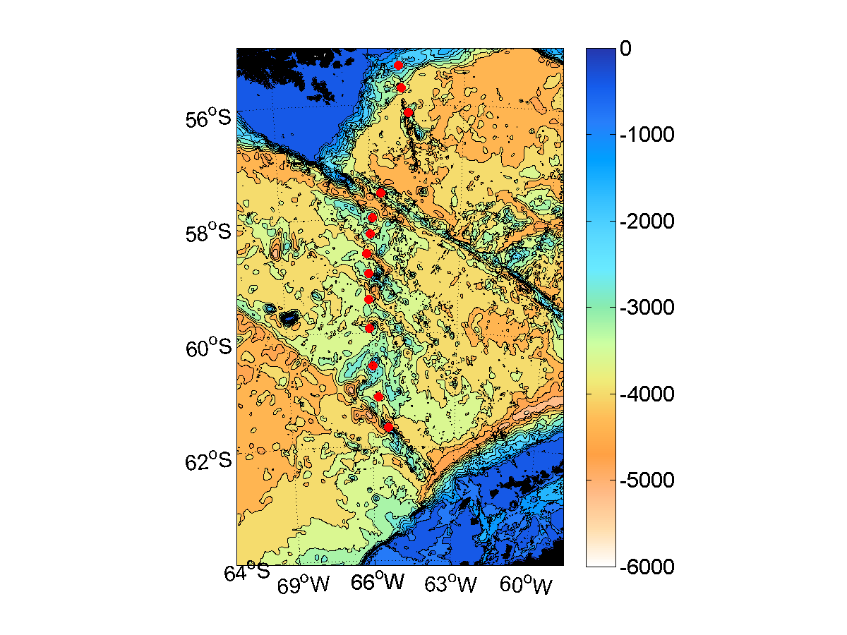
Fig. 2. Stations in Drake Passage, along the Pacific-Antarctic Ridge and Argentine continental slope (red dots). The bathymetry contours are from 0 to 6000 m, every 400 m.
The three remaining RAFOS floats – one shallow and two deep - were deployed along this transect south of the Polar Front. The 6th and last EM-APEX float was deployed near these RAFOS floats – it’s launch position is shown in Fig. 3. The Polar Front is between the second and third stations to the north, according to the temperature at the shallow temperature minimum.
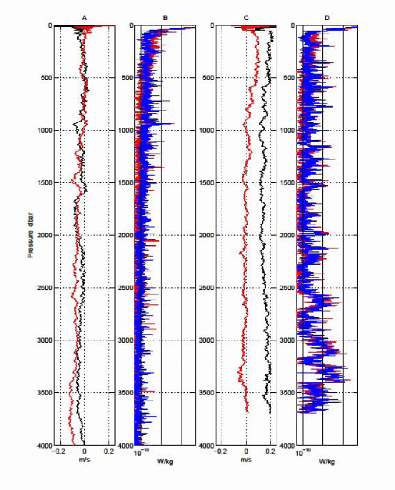
Fig. 3. Vertical profiles of absolute horizontal velocity (panels A and C) and the turbulent kinetic energy dissipation rate (panels B and D) from HRP deployments 40 in the region about the tracer patch and 41 in the Drake Passage. The zonal velocity is shown as black curves and the meridional component in red. Dissipation estimates from the two shear probes on the instrument shown in red and blue are plotted on a semi-logarithmic scale with each whole decade marked.
Seventeen sets of 6 RAFOS floats each were deployed at 20-mile spacing from 56 S to 61-20 S along 105 W during the survey, with three deep floats (neutral density = 1027.9 kg/m3) and three shallow ones (1027.3 kg/m3) at each station (Figs. 1 and 4). CTD casts were done at every other float station with 1800-meter XBTs at the intervening float stations. Twenty shallow floats that were of a new design came to the surface shortly after deployment due to a manufacturer’s oversight. All but one of the other floats are still down as far as is known, and presumably performing their 2-year mission.
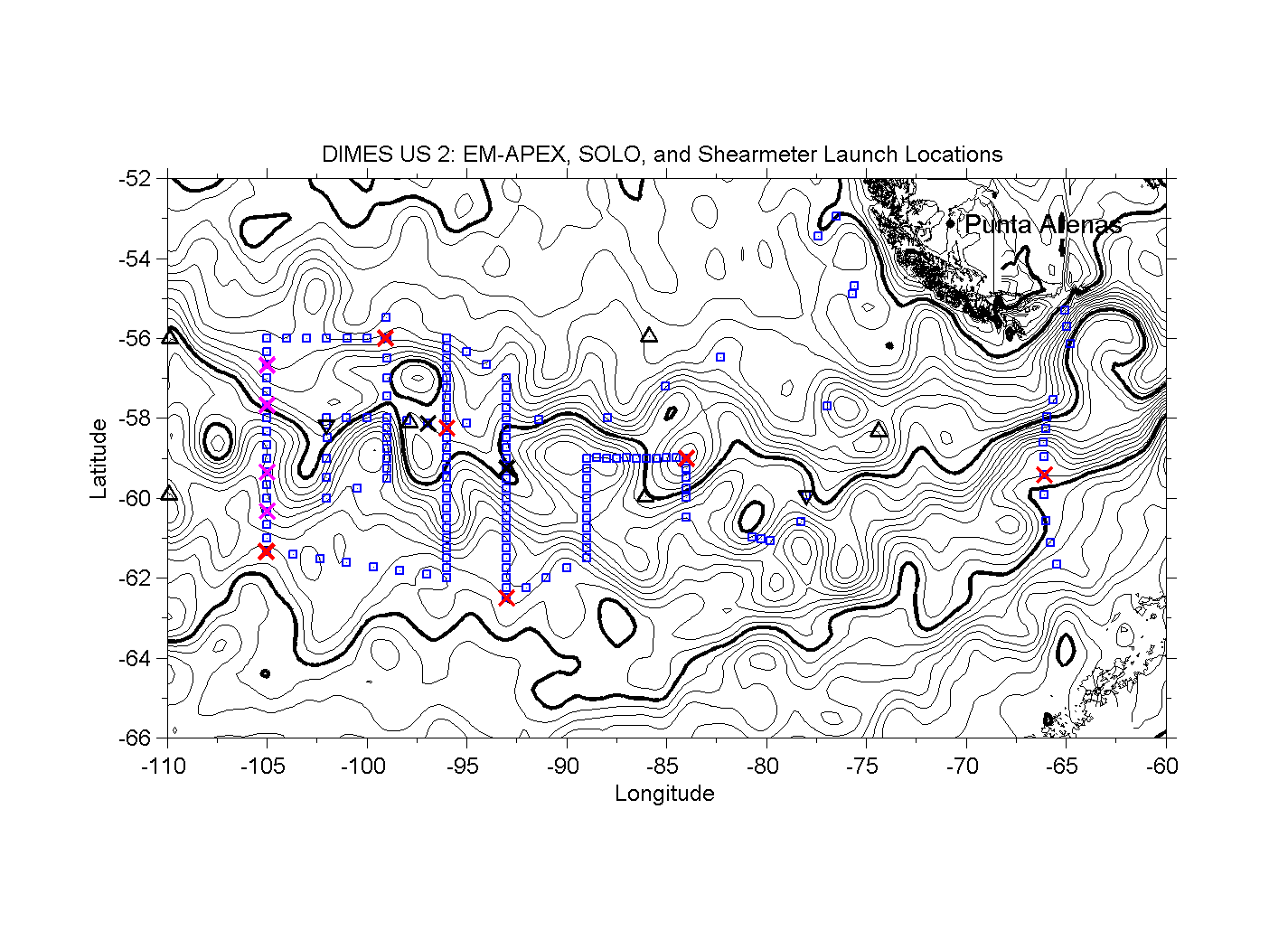
Fig. 4. Float launch positions. Six RAFOS floats were launched at each of the stations along 105 W. Three RAFOS floats were also released in Drake Passage at the red ‘x’. The magenta ‘x’s indicate SOLO floats, the red ‘x’s indicate EM-APEX, and the two black ‘x’s indicate Shearmeters – the one at 97 W executed a 12-day mission; the mission duration for the one at 93 W is 365 days. The triangles indicate the positions of the sound sources. The contours indicate absolute dynamic topography, with a contour interval of 5 cm.
Four SOLO floats and an EM-APEX float were also deployed along 105 W (Fig. 4). The SOLO floats are equipped with RAFOS receivers and should enable monitoring of the performance of the sound sources. Three other EM-APEX floats were deployed in the region of the tracer survey (Fig. 4) in addition to the one in Drake Passage mentioned earlier. Two sound sources were deployed on moorings early in the cruise to supplement the array of sound sources deployed in 2009 (Fig. 1).
A shearmeter was deployed for a 12-day test run early in the cruise (see Fig. 4 for location). It performed well except that its active ballasting mechanism was not activated and it settled at a pressure a little less than 1000 dbar for its mission. Its communication system failed shortly after coming to the surface so that we could not recover it. A second shearmeter was deployed for a 365-day mission, programmed to seek an isothermal surface with its active ballasting system (see Fig. 2 for location). This one has not been heard from and is presumed to be on its mission. A third shearmeter was deployed, programmed to seek an isopycnal surface. It went too deep, released its drop-weight and came to the surface a few hours after deployment. Unfortunately, we were too far away to reach it before nightfall by the time we had resolved its position.
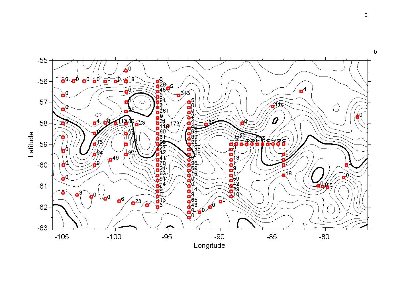
Fig. 5. Map of the tracer stations, with column integrals in units of 10-2 nmol/m2. The triangles indicate the positions of the sound sources. The contours indicate absolute dynamic topography (ADT), with a contour interval of 5 cm. The bold contour near 59 S is just north of the ADT of the tracer release in 2009.
The survey of tracer, hydrography, fine structure and microstructure in the SE Pacific sector of the Antarctic Circumpolar Current, between 78 W and 105 W, was completed on 24 February 2010. Stations that actually found tracer commenced on 27 January and ended on 24 February, and so took 29 days. Fig. 5 shows the station locations and the column integral of tracer found at each station. The tracer distribution is clearly streaky at this time (Figs 6), but it was still possible to obtain accurate mean vertical profiles (Figs. 7 and 8) and a fair idea of where the tracer patch was located. The diapycnal diffusivity calculated from the increase in rms width of the tracer patch between injection in February 2009 and February 2010 is 1.3 x 10⁻⁵ m2/s. Low dissipation rates from the microstructure profilers, and low shear from the profilers and from the LADCP are consistent with this value. Fig. 3 shows an example of velocity and dissipation profiles from the region of the tracer patch as well as an example from the Drake Passage crossing.
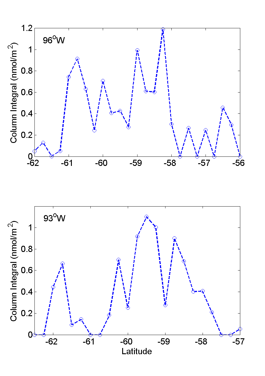
Fig. 6. Column integral of tracer along 96 W and 93 W. The station locations can be seen in Fig. 4.
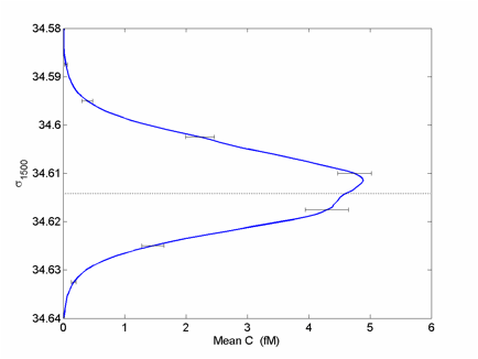
Fig. 7. Mean tracer concentration versus potential density, referenced to 1500 dbar, for all the tracer stations.
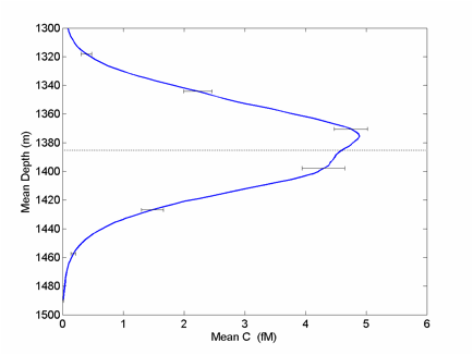
Fig. 8. Mean tracer concentration versus mean depth derived from the mean depth/potential density relation (solid line). The dashed line shows a Gaussian fit to the mean profile